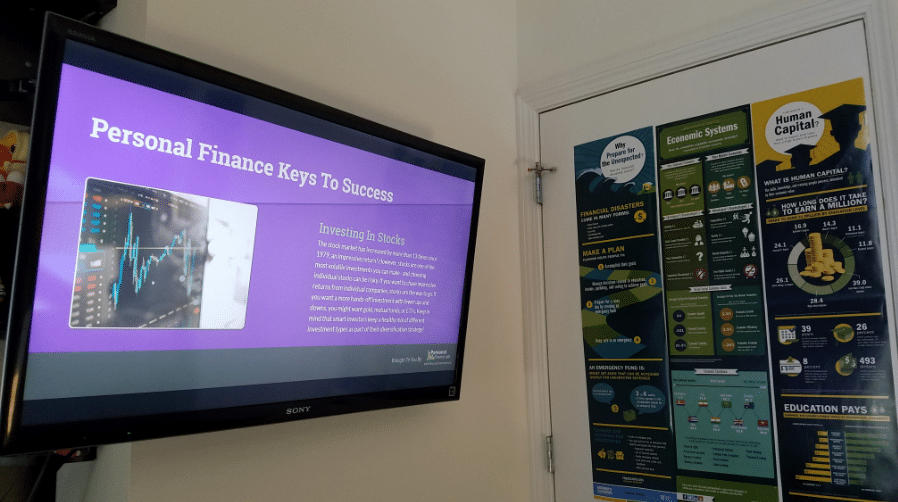
We work with hundreds of schools around the country to take their Personal Finance, Economics, and Business classes to the next level. Over the last few years, more and more schools are using our Personal Budgeting Game, our customizable Stock Market Game, and our curriculum library to start building Finance Lab. Eventually they add on the hardware (scrolling stock tickers and Wall Street-style LCD screens) to change their classroom into the most popular room at their school.
No two schools are the same, and so every lab space is different. However, all successful labs have some combination of these elements – the PersonalFinanceLab.com site license which includes a Budget Game and a Stock Game, an LCD MarketBoard displays, scrolling LED tickers, and fun, educational posters. Here is what you need to know about each when planning out your successful lab:
PersonalFinanceLab.com License
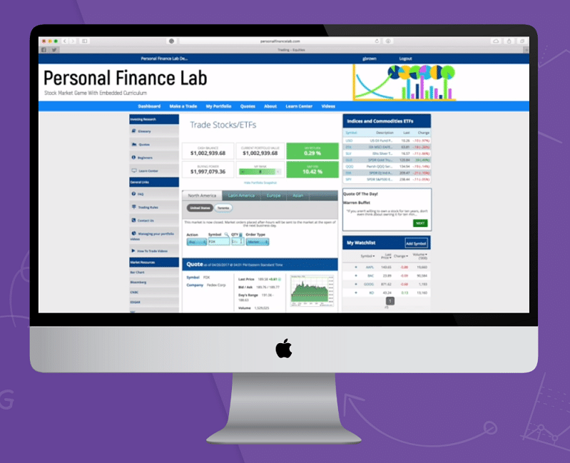
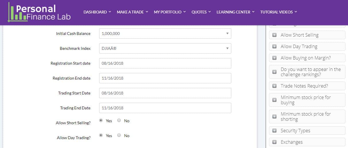
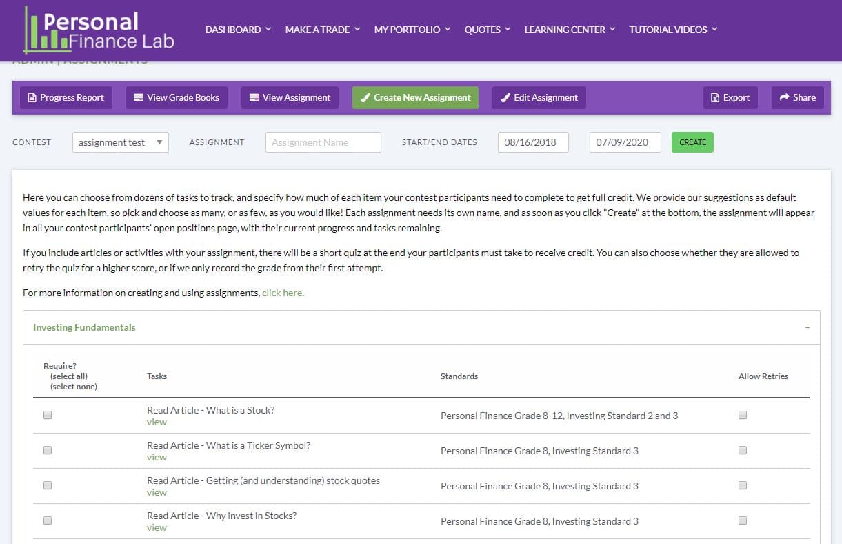
The PersonalFinanceLab.com site license is the starting point for any Personal Finance, Business, or Economics class. This gives your classes access to the PersonalFinanceLab.com Personal Budgeting Game, our customizable Stock Market Game, curriculum, assessments, teacher reports, research tools, and Investing101 course.
The Budget Game, the Stock Game, and the curriculum are endlessly customizable, with plenty of quick-start settings to help you dive in. This will let you run your class stock contest (and keeping engaged in the class rankings), while students work through their Personal Finance, Economics, Accounting, or Business lessons that you choose each week. Each lesson ends with a quiz, and you can automatically add unit assessments to track overall progress (with plenty of reporting tools!) This is also the fastest and easiest part of your lab to launch – your classes can be up and running in as little as 24 hours – including a live webinar with the PFinLab team to help you get started.
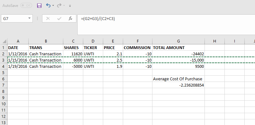
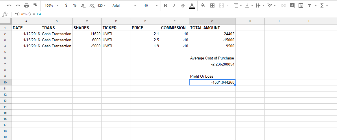
Pricing
Individual/Student Accounts for less than 100 students
- Cost: $10/student for either our stock game or budget game (both include our full curriculum library)
- Or get both the stock AND budget game for just $15 / student!
- Ideal for teachers that need less than 100 accounts per year
- Order Now and pay with a credit card or request an invoice.
Single Class License
- Covers: up to 60 students per year
- Cost: $595 / year for either the Budget Game or the Stock Game
- or $895 / year for BOTH the Budget Game and the Stock Game
- Perfect For: Smaller schools with one or two teachers teaching financial literacy and business
- Order Now and pay with a credit card or request an invoice.
Micro Site License
- Covers: up to 100 students per year
- Cost: $995 / year for either the Budget Game or the Stock Game
- or $1,495 / year for BOTH the Budget Game and the Stock Game
- Perfect For: Smaller schools with one or two teachers teaching financial literacy and business
- Order Now and pay with a credit card or request an invoice.
Mini Site License
- Covers: up to 250 students per year
- Cost: $1995 / year for either the Budget Game or the Stock Game
- or $2,995 / year for BOTH the Budget Game and the Stock Game
- Perfect For: Medium schools with multiple economics, personal finance, and business classes
- Order Now and pay with a credit card or request an invoice.
Full Site License
- Covers: up to 1,000 students / year
- Cost: $3,995 / year
- or $5,995 / year for BOTH the Budget Game and the Stock Game
- Perfect For: Large schools with a focus on business and finance education, and schools that run school-wide investing challenges (Prizes are available)
- Order Now and pay with a credit card or request an invoice.
If you want to launch your lab quickly and cheaply this semester, you can’t go wrong with the Single Class license, and upgrade once more funds become available.
Learn More about the PersonalFinanceLab stock game and curriculum!
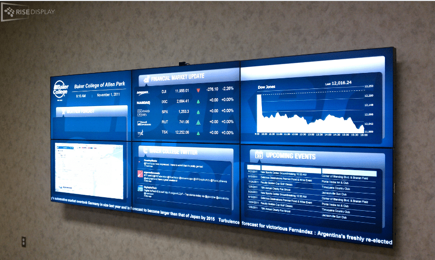
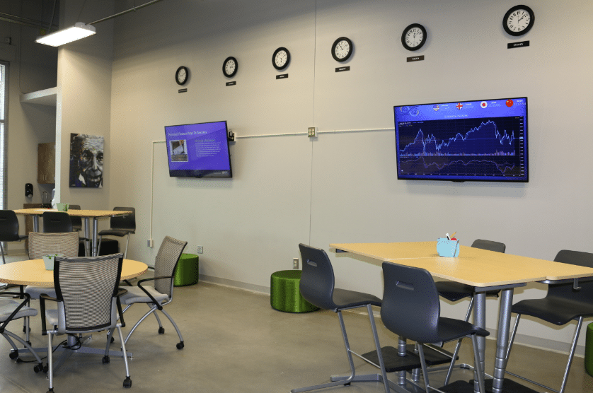
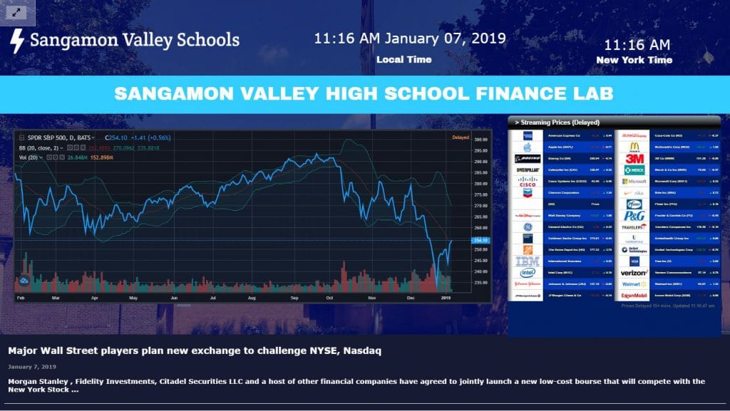
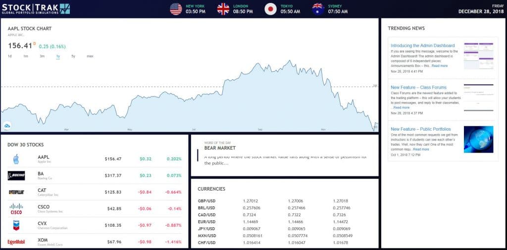
LCD “MarketInsight” Displays

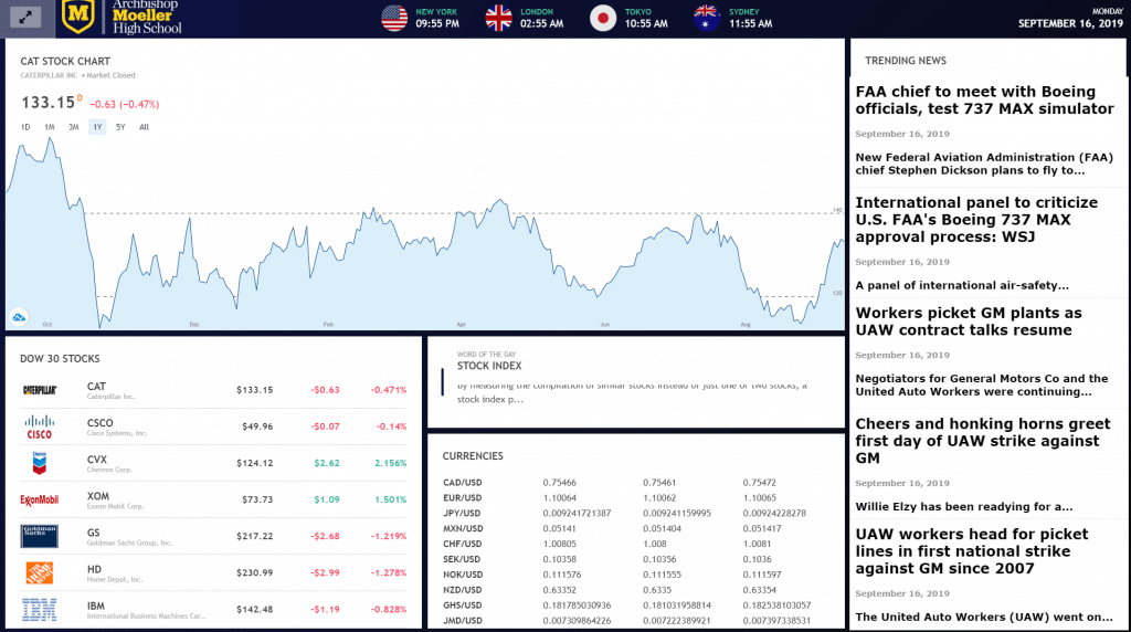
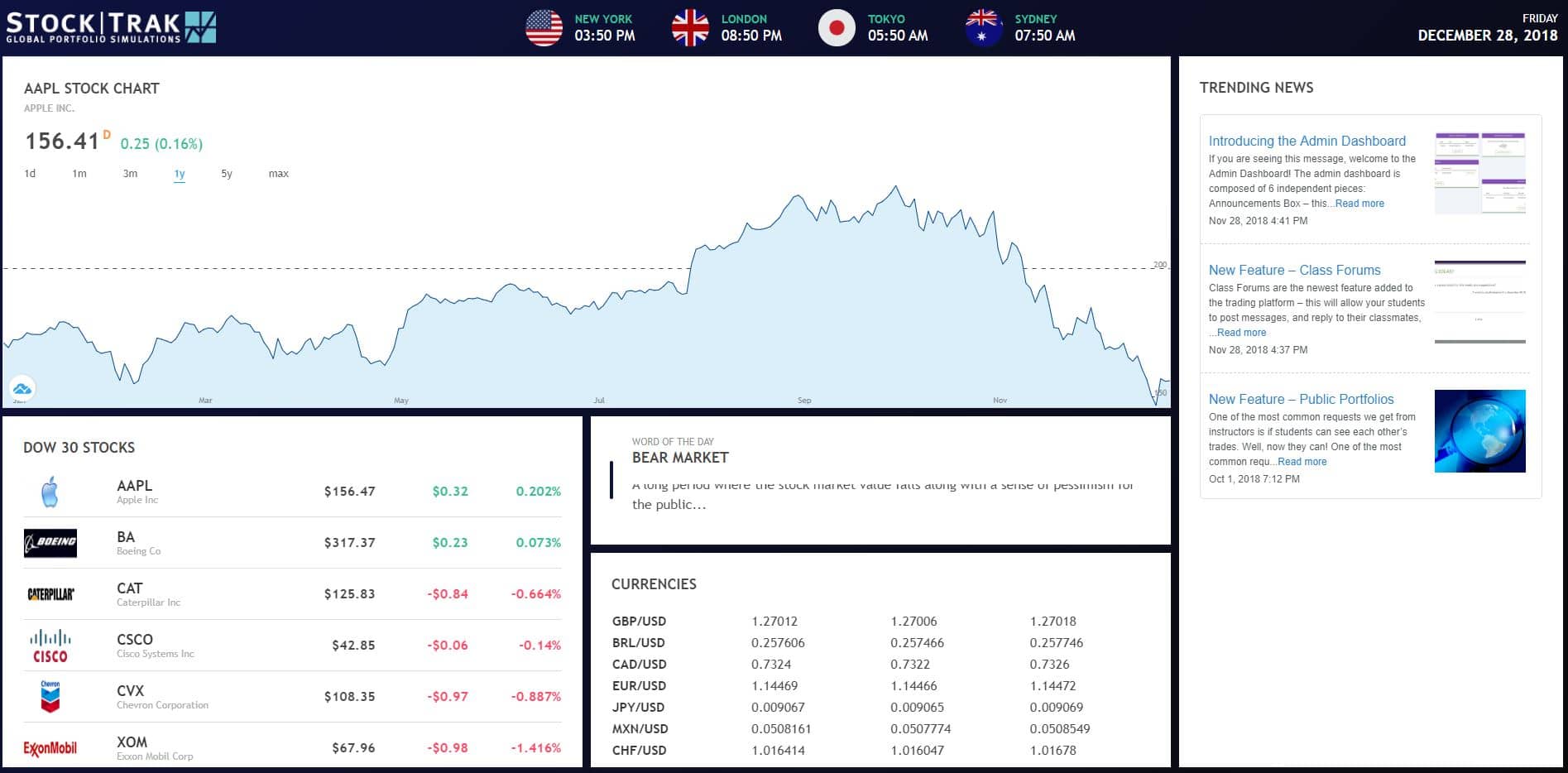
The MarketInsight display is one of the fundamental pieces of any Finance Lab. This is an LCD screen that can rotate several financial “widgets” for your classes. The coolest part is that each MarketInsight is fully configurable – you choose what you want displayed! Click Here to see some options of what you can put on your MarketInsight Display.
There are two ways to upgrade to a MarketInsight – upgrade an existing TV, or order a commercial-grade screen.
MarketInsight Installation Tip:
MarketInsight draw a lot of attention – so keep this in mind when installing in your classroom! MarketInsight are best positioned at the sides or the rear of the room to avoid them becoming a distraction during instruction time.
Upgrading a TV
To upgrade a TV you already have at your school (or one you buy specifically for this purpose), you will need to order a $99 “Intel Stick”, which plugs into any HDMI port. This will connect to your school’s WiFi and the data feed to display your widgets. If you decide to upgrade a TV, remember to turn the screens off at the end of the day to avoid long-term screen burn.
Cost: $99 for each “Intel Stick”, plus $360/year for up to 3 screens for the data feed.
Commercial-Grade Display
Schools building a completely dedicated lab space may better be served by commercial-grade LCD display screens. These are typically a bit more expensive than a standard TV, but are designed to stay on for years at a time without any screen-burn. They are used both inside the classroom, as well as in the school hallways where they are expected to stay on regularly overnight. The purpose-built displays come with their own media players, so there is no need for an “Intel Stick” with this route.
Cost: A 48″ display costs about $1350, including shipping. Larger screens are slightly more expensive. This also requires a $360/year data feed, which covers up to 3 screens.
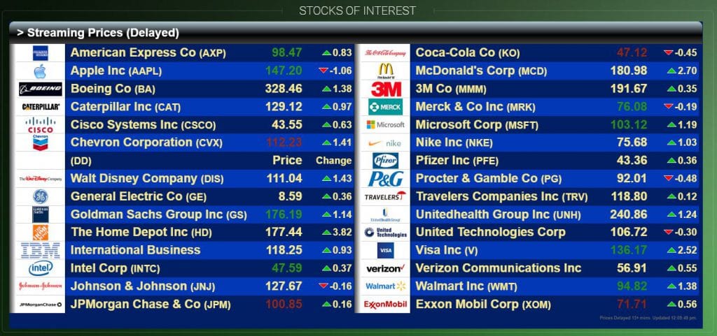
Scrolling LED Tickers
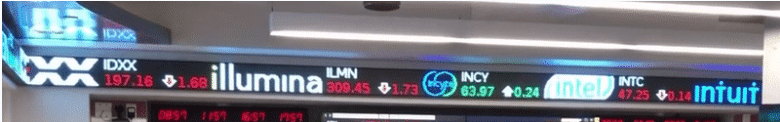
Scrolling LED tickers are the crown jewel of any lab. These bring live market data into your classroom, making it the most exciting room at the school. If you do have an LED ticker, you will want to show it off – try to position it in the room so that it is visible from outside, but not at the very front of the class (to avoid it becoming a distraction).
In fact, many schools with LED tickers opt to either have windows on the classroom to make it completely visible from the hallway, or even install a second ticker in the hallway to grab the attention of passing students (and visiting parents). Tickers work best when you have drop-ceilings; they will need a standard power supply AND a hard-wire ethernet internet connection (they will not connect to your school’s WiFi)
See our gallery of recently-completed labs!
Cost: An 8-foot ticker costs about $5,200, 16-foot tickers cost about $10,000. Larger tickers are available in 4-foot increments. Each ticker also requires its own $499/year data feed.
Free Posters

Educational Personal Finance and Economics posters are an awesome way to spice up your classroom, and the first step in its transformation into a Finance Lab. Best of all, the best posters are free for schools thanks to the Federal Reserve in Atlanta!
There are over 15 different posters to choose from – pick which ones you like, and they will ship directly to your school, free of charge. These posters are a free (and super easy) way to “Set the mood” of your classroom – making it one of the fundamental building blocks of a Lab.
Click Here To Order Your Posters
Get More Information
Have more questions? Ready to launch your lab? Let us know and we’ll be happy to help!

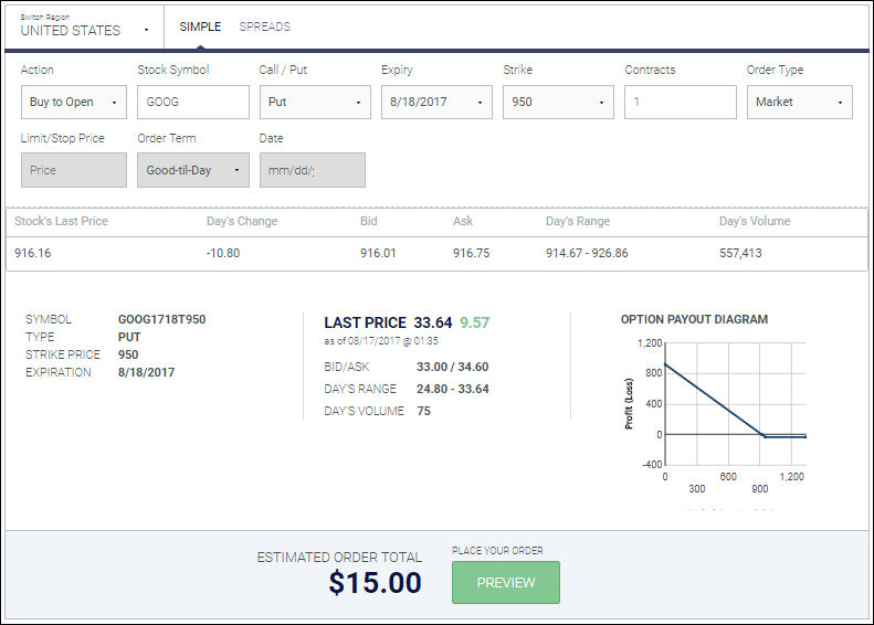
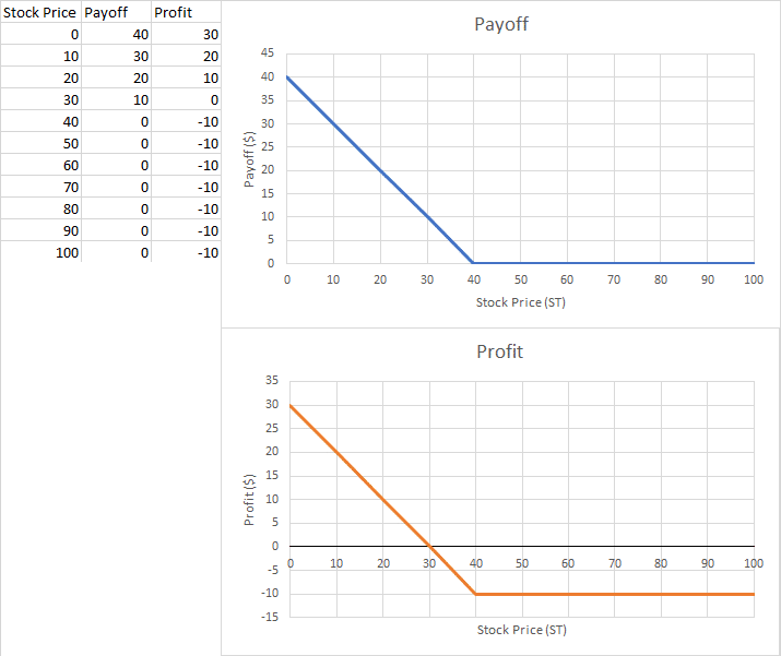
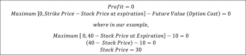
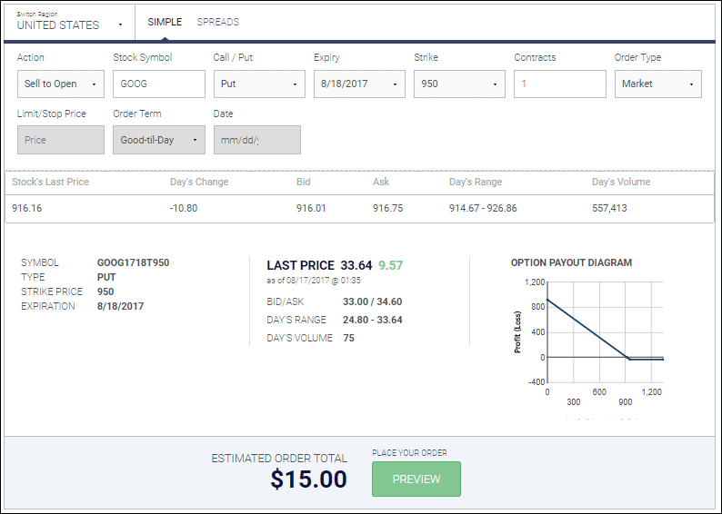
 Imagine two farmers – Alice and Bob. Alice and Bob both have farms located 15 miles away from a major city, and both have about the same quality of soil. If they both grow corn in the same year, they will produce about the same amount, and earn the same income. In this example, neither Alice nor Bob has any comparative advantage.
 If Alice always re-invests half of her income into her business, but Bob does not, within a few years Alice’s machines and tools will be a lot more up-to-date and productive than Bob’s.


 There are a few ways to calculate GDP, but the easiest measurement looks at consumption, investment, government activity, and net exports.
 GDP increases when output increases. When we look at how much a country could potentially produce in a given year, if its resources were all being utilized to the maximum, we would consider:
 Think of it this way: England spent over a hundred years and the equivalent of billions of dollars building railroads all over their country to help speed up trade. Every year, companies would spend millions to make small improvements to the rail engine technology. This slowly improved their technology, quantity, and quality of capital goods.